Yo I heard you like bootstraps
28 Sep 2017Often an estimator is biased in finite samples. For example, say that we try to estimate $\mathrm{E}[x]^4$ by raising the sample mean of $x$ to the fourth power. By Jensen’s inequality, the estimate will be positively biased. We can achieve an asmptotic refinement and reduce the bias of the estimator with a bootstrapped bias correction. In case our bootstrap estimate of the bias is biased, we can bootstrap a bias correction to the bootstrapped bias correction, for a higher-order asymptotic refinement. If your bias correction to the bias correction is biased, you can… well, you know.
For the purpose of illustration I’ll draw data $N(0, 1)$, but in general we won’t know the data-generating process.
import numpy as np
from matplotlib import pyplot as plt
from math import exp
%matplotlib inline
np.random.seed(92817)

# our estimator
def g(vec):
    return np.mean(vec)**4

mean = 0
true_answer = g(mean)
n_obs = 10
x = np.random.normal(mean, 1, n_obs)
estimated_answer = g(x)
print('True answer ', true_answer)

print('Estimated answer ', estimated_answer)
True answer  0.0
Estimated answer  1.55064636855e-08
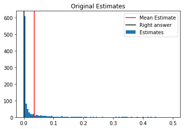
Alright, that was pretty close, but the estimates usually aren’t so close to the population value. Let’s take a look at the distribution of estimates:
n_x_draws = 1000
x_draws = np.random.normal(mean, 1, (n_x_draws, n_obs))
estimates = np.apply_along_axis(g, 1, x_draws)
np.mean(estimates)
0.035422624583334866
The mean estimate is too high, because our estimator is concave. That is, if we draw $x_1, \dots, x_K$, then $\mathrm{E} \left[ g \left( \frac{1}{K} \sum_i x_i \right) \right] > \mathrm{E} \left[ g \left( \mathrm{E}[x] \right) \right]$.
We can estimate a bias correction using the bootstrap. If x(b) is a bootstrap draw from x, then
$ \mathrm{E} \left[ g \left( \frac{1}{K} \sum_i x(b)_i \right) \right] - \mathrm{E} \left[ g \left( \frac{1}{K} \sum_i x_i \right) \right] = \mathrm{E} \left[ g \left( \frac{1}{K} \sum_i x_i \right) \right] - \mathrm{E} \left[ g\left( \mathrm{E}[x] \right) \right]$,
up to $O(n^{-2})$.
Why does this work? For a sufficiently high-dimensional x, the bootstrap distribution of x will be similar to the true distribution of x, but centered at the sample mean of x rather than at zero. Thus, the Taylor expansions of g(mean(x(b))) around g(mean(x)) and of g(mean(x)) around $\mathrm{E}[x]$ both have first terms that are zero in expectation and a similar second term, which depends on $g’’$.
def get_bootstrap_bias_correction(estimator, data, n_draws):
    estimate = estimator(data)
    bootstrap_estimate_sum = 0
    for _ in range(n_draws):
        bootstrap_estimate_sum += \
            estimator(np.random.choice(data, len(data)))
    return bootstrap_estimate_sum / n_draws - estimate

def get_bias_corrected_estimate(estimator, data, n_draws):
    estimate = estimator(data)
    bias_correction = get_bootstrap_bias_correction(estimator, data, n_draws)
    return estimate - bias_correction

n_boot_draws = 1000
bias_corrected = get_bias_corrected_estimate(g, x, n_boot_draws)
print('One bias-corrected estimate', bias_corrected)
One bias-corrected estimate -0.0390486143447
Let’s do the same thing for each of our x’s, so we can see how well the bias correction does on average.
bias_corrected_all = np.apply_along_axis(
    lambda x: get_bias_corrected_estimate(g, x, n_boot_draws),
    1, x_draws)
Here’s a histogram:
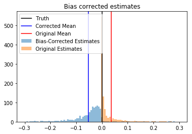
So I bootstrapped your bootstrap
As expected, the bias-corrected estimates are lower, but unfortunately they’re actually more biased. Even though the bias correction ought to work well in large samples, our estimator of the bias is biased in the small n=10 samples we have. What to do? I guess we could bootstrap a bias correction to the bootstrapped bias correction.
def get_double_bias_corrected_estimate(estimator, data, n_draws):
    estimate = estimator(data)
    bias_correction = get_bias_corrected_estimate(
        lambda z: get_bootstrap_bias_correction(estimator, z, n_draws),
        data, n_draws
    )
    return estimate - bias_correction
The double bias correction will call the estimator n_draws^2 times. Let’s just call it with sqrt(n_draws) so that it takes as long as the original bias correction.
small_n_draws = int(n_boot_draws**.5)
double_corrected_estimates = np.apply_along_axis(
    lambda x: get_double_bias_corrected_estimate(g, x, small_n_draws),
    1, x_draws)
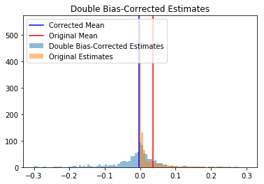
The mean double bias-corrected estimate is now quite close to the true mean: We’ve created an unbiased estimator, albeit at the expense of greater variance and MSE.
print('Bias of original', np.mean(estimates - true_answer))
print('Bias of double-corrected', np.mean(double_corrected_estimates - true_answer))
print('\nVariance of original', np.var(estimates))
print('Variance of double-corrected', np.var(double_corrected_estimates))
print('\nMSE of original',
      np.mean((estimates - true_answer)**2))
print('MSE of double-corrected',
      np.mean((double_corrected_estimates - true_answer)**2))
Bias of original 0.0354226245833
Bias of double-corrected -0.00300251292168

Variance of original 0.0183016628265
Variance of double-corrected 0.0324580890936

MSE of original 0.0195564251588
MSE of double-corrected 0.0324671041774
So you can bootstrap your bootstrapped bootstrap
Can we recurse?
def get_recursive_bias_correction(estimator, data, n_draws, n_layers):
    assert n_layers >= 1
    if n_layers == 1:
        f = estimator
        return get_bootstrap_bias_correction(f, data, n_draws)
    else:
        def f(z):
            return get_recursive_bias_correction(estimator, z,
                                                 n_draws, n_layers - 1)
        return get_bias_corrected_estimate(f, data, n_draws)
Let’s check that this gives the same answers as our original bias corrections.
new_first_correction = np.apply_along_axis(
    lambda z: get_recursive_bias_correction(g, z, 100, 1),
    1, x_draws)

old_first_correction = np.mean(estimates - bias_corrected_all)
print('First mean', np.mean(old_first_correction))
print('New mean', np.mean(new_first_correction))
First mean 0.0876449721805
New mean 0.0864229782315
new_second_correction = np.apply_along_axis(
    lambda z: get_recursive_bias_correction(g, z, 30, 2),
    1, x_draws)

old_second_correction = estimates - double_corrected_estimates
print('First mean', np.mean(old_second_correction))
print('New mean', np.mean(new_second_correction))
First mean 0.038425137505
New mean 0.0379599582098